Saturday, May 15, 2010

Relationship to continuum mechanics

Fluid mechanics is a subdiscipline of continuum mechanics, as illustrated in the following table.

Continuum mechanics the study of the physics of continuous materials Solid mechanics: the study of the physics of continuous materials with a defined rest shape. Elasticity: which describes materials that return to their rest shape after an applied stress.
Plasticity: which describes materials that permanently deform after a large enough applied stress. Rheology: the study of materials with both solid and fluid characteristics
Fluid mechanics: the study of the physics of continuous materials which take the shape of their container. Non-Newtonian fluids
Newtonian fluids

In a mechanical view, a fluid is a substance that does not support shear stress; that is why a fluid at rest has the shape of its containing vessel. A fluid at rest has no shear stress.

Assumptions

Like any mathematical model of the real world, fluid mechanics makes some basic assumptions about the materials being studied. These assumptions are turned into equations that must be satisfied if the assumptions are to be held true. For example, consider an incompressible fluid in three dimensions. The assumption that mass is conserved means that for any fixed closed surface (such as a sphere) the rate of mass passing from outside to inside the surface must be the same as rate of mass passing the other way. (Alternatively, the mass inside remains constant, as does the mass outside). This can be turned into an integral equation over the surface.

Fluid mechanics assumes that every fluid obeys the following:

  • Conservation of mass
  • Conservation of momentum
  • The continuum hypothesis, detailed below.

Further, it is often useful (and realistic) to assume a fluid is incompressible – that is, the density of the fluid does not change. Liquids can often be modelled as incompressible fluids, whereas gases cannot.

Similarly, it can sometimes be assumed that the viscosity of the fluid is zero (the fluid is inviscid). Gases can often be assumed to be inviscid. If a fluid is viscous, and its flow contained in some way (e.g. in a pipe), then the flow at the boundary must have zero velocity. For a viscous fluid, if the boundary is not porous, the shear forces between the fluid and the boundary results also in a zero velocity for the fluid at the boundary. This is called the no-slip condition. For a porous media otherwise, in the frontier of the containing vessel, the slip condition is not zero velocity, and the fluid has a discontinuous velocity field between the free fluid and the fluid in the porous media (this is related to the Beavers and Joseph condition).

The continuum hypothesis

Fluids are composed of molecules that collide with one another and solid objects. The continuum assumption, however, considers fluids to be continuous. That is, properties such as density, pressure, temperature, and velocity are taken to be well-defined at "infinitely" small points, defining a REV (Reference Element of Volume), at the geometric order of the distance between two adjacent molecules of fluid. Properties are assumed to vary continuously from one point to another, and are averaged values in the REV. The fact that the fluid is made up of discrete molecules is ignored.

The continuum hypothesis is basically an approximation, in the same way planets are approximated by point particles when dealing with celestial mechanics, and therefore results in approximate solutions. Consequently, assumption of the continuum hypothesis can lead to results which are not of desired accuracy. That said, under the right circumstances, the continuum hypothesis produces extremely accurate results.

Those problems for which the continuum hypothesis does not allow solutions of desired accuracy are solved using statistical mechanics. To determine whether or not to use conventional fluid dynamics or statistical mechanics, the Knudsen number is evaluated for the problem. The Knudsen number is defined as the ratio of the molecular mean free path length to a certain representative physical length scale. This length scale could be, for example, the radius of a body in a fluid. (More simply, the Knudsen number is how many times its own diameter a particle will travel on average before hitting another particle). Problems with Knudsen numbers at or above unity are best evaluated using statistical mechanics for reliable solutions.

Navier–Stokes equations

The Navier–Stokes equations (named after Claude-Louis Navier and George Gabriel Stokes) are the set of equations that describe the motion of fluid substances such as liquids and gases. These equations state that changes in momentum (force) of fluid particles depend only on the external pressure and internal viscous forces (similar to friction) acting on the fluid. Thus, the Navier–Stokes equations describe the balance of forces acting at any given region of the fluid.

The Navier–Stokes equations are differential equations which describe the motion of a fluid. Such equations establish relations among the rates of change the variables of interest. For example, the Navier–Stokes equations for an ideal fluid with zero viscosity states that acceleration (the rate of change of velocity) is proportional to the derivative of internal pressure.

This means that solutions of the Navier–Stokes equations for a given physical problem must be sought with the help of calculus. In practical terms only the simplest cases can be solved exactly in this way. These cases generally involve non-turbulent, steady flow (flow does not change with time) in which the Reynolds number is small.

For more complex situations, such as global weather systems like El Niño or lift in a wing, solutions of the Navier–Stokes equations can currently only be found with the help of computers. This is a field of sciences by its own called computational fluid dynamics.

General form of the equation

The general form of the Navier–Stokes equations for the conservation of momentum is:

\rho\frac{D\mathbf{v}}{D t} = \nabla\cdot\mathbb{P} + \rho\mathbf{f}

where

  • \rho\ is the fluid density,
  • \frac{D}{D t} is the substantive derivative (also called the material derivative),
  • \mathbf{v} is the velocity vector,
  • \mathbf{f} is the body force vector, and
  • \mathbb{P} is a tensor that represents the surface forces applied on a fluid particle (the comoving stress tensor).

Unless the fluid is made up of spinning degrees of freedom like vortices, \mathbb{P} is a symmetric tensor. In general, (in three dimensions) \mathbb{P} has the form:

\mathbb{P} = \begin{pmatrix} \sigma_{xx} &  \tau_{xy} & \tau_{xz} \\ \tau_{yx} &  \sigma_{yy} & \tau_{yz} \\ \tau_{zx} &  \tau_{zy} & \sigma_{zz} \end{pmatrix}

where

  • \sigma\ are normal stresses,
  • \tau\ are tangential stresses (shear stresses).

The above is actually a set of three equations, one per dimension. By themselves, these aren't sufficient to produce a solution. However, adding conservation of mass and appropriate boundary conditions to the system of equations produces a solvable set of equations.

Newtonian versus non-Newtonian fluids

A Newtonian fluid (named after Isaac Newton) is defined to be a fluid whose shear stress is linearly proportional to the velocity gradient in the direction perpendicular to the plane of shear. This definition means regardless of the forces acting on a fluid, it continues to flow. For example, water is a Newtonian fluid, because it continues to display fluid properties no matter how much it is stirred or mixed. A slightly less rigorous definition is that the drag of a small object being moved slowly through the fluid is proportional to the force applied to the object. (Compare friction). Important fluids, like water as well as most gases, behave — to good approximation — as a Newtonian fluid under normal conditions on Earth.[2]

By contrast, stirring a non-Newtonian fluid can leave a "hole" behind. This will gradually fill up over time – this behaviour is seen in materials such as pudding, oobleck, or sand (although sand isn't strictly a fluid). Alternatively, stirring a non-Newtonian fluid can cause the viscosity to decrease, so the fluid appears "thinner" (this is seen in non-drip paints). There are many types of non-Newtonian fluids, as they are defined to be something that fails to obey a particular property — for example, most fluids with long molecular chains can react in a non-Newtonian manner.[2] Equations for a Newtonian fluid

The constant of proportionality between the shear stress and the velocity gradient is known as the viscosity. A simple equation to describe Newtonian fluid behaviour is

\tau=-\mu\frac{dv}{dx}

where

τ is the shear stress exerted by the fluid ("drag")
μ is the fluid viscosity – a constant of proportionality
\frac{dv}{dx} is the velocity gradient perpendicular to the direction of shear

For a Newtonian fluid, the viscosity, by definition, depends only on temperature and pressure, not on the forces acting upon it. If the fluid is incompressible and viscosity is constant across the fluid, the equation governing the shear stress (in Cartesian coordinates) is

\tau_{ij}=\mu\left(\frac{\partial v_i}{\partial x_j}+\frac{\partial v_j}{\partial x_i} \right)

where

τij is the shear stress on the ith face of a fluid element in the jth direction
vi is the velocity in the ith direction
xj is the jth direction coordinate

If a fluid does not obey this relation, it is termed a non-Newtonian fluid, of which there are several types.

Among fluids, two rough broad divisions can be made: ideal and non-ideal fluids. An ideal fluid really does not exist, but in some calculations, the assumption is justifiable. An Ideal fluid is non viscous- offers no resistance whatsoever to a shearing force.

One can group real fluids into Newtonian and non-Newtonian. Newtonian fluids agree with Newton's law of viscosity. Non-Newtonian fluids can be either plastic, bingham plastic, pseudoplastic, dilatant, thixotropic, rheopectic, viscoelatic.

Motion (physics)

In physics, motion is change of location or position of an object with respect to time. Change in motion is the result of an applied force. Motion is typically described in terms of velocity also seen as speed, acceleration, displacement, and time.[1] An object's velocity cannot change unless it is acted upon by a force, as described by Newton's first law also known as Inertia. An object's momentum is directly related to the object's mass and velocity, and the total momentum of all objects in a closed system (one not affected by external forces) does not change with time, as described by the law of conservation of momentum.

A body which does not move is said to be at rest, motionless, immobile, stationary, or to have

Motion involves change in position, such as in this perspective of rapidly leaving Yongsan Station

constant (time-invariant) position.

Motion is always observed and measured relative to a frame of reference. As there is no absolute reference frame, absolute motion cannot be determined; this is emphasised by the term relative motion.[2] A body which is motionless relative to a given reference frame, moves relative to infinitely many other frames. Thus, everything in the universe is moving.[3]

More generally, the term motion signifies any spatial and/or temporal change in a physical system. For example, one can talk about motion of a wave or a quantum particle (or any other field) where the concept location does not apply.

Laws of Motion

In physics, motion in the universe is described through two sets of apparently contradictory laws of mechanics. Motions of all large scale and familiar objects in the universe (such as projectiles, planets, cells, and humans) are described by classical mechanics. Whereas the motion of very small atomic and sub-atomic sized objects is described by quantum mechanics.

Classical mechanics

Classical mechanics
\mathbf{F} = \frac{\mathrm{d}}{\mathrm{d}t}(m \mathbf{v})
Newton's Second Law
History of ...
Fundamental concepts
Space · Time · Velocity · Speed · Mass · Acceleration · Gravity · Force · Torque / Moment / Couple · Momentum · Angular momentum · Inertia · Moment of inertia · Reference frame · Energy · Kinetic energy · Potential energy · Mechanical work · Virtual work · D'Alembert's principle

Classical mechanics is used for describing the motion of macroscopic objects, from projectiles to parts of machinery, as well as astronomical objects, such as spacecraft, planets, stars, and galaxies. It produces very accurate results within these domains, and is one of the oldest and largest subjects in science, engineering and technology.

Classical mechanics is fundamentally based on Newton's Laws of Motion. These laws describe the relationship between the forces acting on a body and the motion of that body. They were first compiled by Sir Isaac Newton in his work Philosophiæ Naturalis Principia Mathematica, first published on July 5, 1687. His three laws are:

  1. In the absence of a net external force, a body either is at rest or moves with constant velocity.
  2. The net external force on a body is equal to the mass of that body times its acceleration; F = ma. Alternatively, force is proportional to the time derivative of momentum.
  3. Whenever a first body exerts a force F on a second body, the second body exerts a force −F on the first body. F and −F are equal in magnitude and opposite in direction.[4]

Newton's three laws of motion, along with his law of universal gravitation, explain Kepler's laws of planetary motion, which were the first to accurately provide a mathematical model or understanding orbiting bodies in outer space. This explanation unified the motion of celestial bodies and motion of objects on earth.

Classical mechanics was later further enhanced by Albert Einstein's special relativity and general relativity. Special relativity explains the motion of objects with a high velocity, approaching the speed of light; general relativity is employed to handle gravitation motion at a deeper level.

Quantum mechanics

Quantum mechanics is a set of principles describing physical reality at the atomic level of matter (molecules and atoms) and the subatomic (electrons, protons, and even smaller particles). These descriptions include the simultaneous wave-like and particle-like behavior of both matter and radiation energy, this described in the wave–particle duality.

In contrast to classical mechanics, where accurate measurements and predictions can be calculated about location and velocity, in the quantum mechanics of a subatomic particle, one can never specify its state, such as its simultaneous location and velocity, with complete certainty (this is called the Heisenberg uncertainty principle).

In addition to describing the motion of atomic level phenomenon, quantum mechanics is useful in understanding some large scale phenomenon such as superfluidity, superconductivity, and biological systems, including the function of smell receptors and the structures of proteins.

List of "imperceptible" human motions

Humans, like all things in the universe are in constant motion,[5] however, aside from obvious movements of the various external body parts and locomotion, humans are in motion in a variety of ways which are more difficult to perceive. Many of these "imperceptible motions" are only perceivable with the help of special tools and careful observation. The larger scales of "imperceptible motions" are difficult for humans to perceive for two reasons: 1) Newton's laws of motion (particularly Inertia) which prevent humans from feeling motions of a mass to which they are connected, and 2) the lack of an obvious frame of reference which would allow individuals to easily see that they are moving.[6] The smaller scales of these motions are too small for humans to sense.

Universe

  • Spacetime (the fabric of the universe) is actually expanding. Essentially, everything in the universe is stretching like a rubber band. This motion is the most obscure as it is not physical motion as such, but rather a change in the very nature of the universe. The primary source of verification of this expansion was provided by Edwin Hubble who demonstrated that all galaxies and distant astronomical objects were moving away from us ("Hubble's law") as predicted by a universal expansion.[7]

Galaxy

  • The Milky Way Galaxy, is hurtling through space at an incredible speed. It is powered by the force left over from the Big Bang. Many astronomers believe the Milky Way is moving at approximately 600 km/s relative to the observed locations of other nearby galaxies. Another reference frame is provided by the Cosmic microwave background. This frame of reference indicates that The Milky Way is moving at around 552 km/s.[8]

Solar System

  • The Milky Way is rotating around its dense galactic center, thus the solar system is moving in a circle within the galaxy's gravity. Away from the central bulge or outer rim, the typical stellar velocity is between 210 and 240 km/s (or about a half-million mi/h).[9]

Earth

  • The Earth is rotating or spinning around its axis, this is evidenced by day and night, at the equator the earth has an eastward velocity of 0.4651 km/s (or 1040 mi/h).[10]
  • The Earth is orbiting around the Sun in an orbital revolution. A complete orbit around the sun takes one year or about 365 days; it averages a speed of about 30 km/s (or 67,000 mi/h).[11]

Continents

  • The Theory of Plate tectonics tells us that the continents are drifting on convection currents within the mantle causing them to move across the surface of the planet at the slow speed of approximately 1 inch (2.54 cm) per year.[12][13] However, the velocities of plates range widely. The fastest-moving plates are the oceanic plates, with the Cocos Plate advancing at a rate of 75 mm/yr[14] (3.0 in/yr) and the Pacific Plate moving 52–69 mm/yr (2.1–2.7 in/yr). At the other extreme, the slowest-moving plate is the Eurasian Plate, progressing at a typical rate of about 21 mm/yr (0.8 in/yr).

Internal body

  • The human heart is constantly contracting to move blood throughout the body. Through larger veins and arteries in the body blood has been found to travel at approximately 0.33 m/s.[15] Though considerable variation exists, and peak flows in the venae cavae have been found to range between 0.1 m/s and 0.45 m/s.[16]
  • The smooth muscles of hollow internal organs are moving. The most familiar would be peristalsis which is where digested food is forced throughout the digestive tract. Though different foods travel through the body at rates, an average speed through the human small intestine is 2.16 m/h or 0.036 m/s.[17]
  • Typically some sound is audible at any given moment, when the vibration of these sound waves reaches the ear drum it moves in response and allows the sense of hearing.
  • The human lymphatic system is constantly moving excess fluids, lipids, and immune system related products around the body. The lymph fluid has been found to move through a lymph capillary of the skin at approximately 0.0000097 m/s.[18]

Cells

The cells of the human body have many structures which move throughout them.

  • Cytoplasmic streaming is a way which cells move molecular substances throughout the cytoplasm.[19]
  • Various motor proteins work as molecular motors within a cell and move along the surface of various cellular substrates such as microtubules. Motor proteins are typically powered by the hydrolysis of adenosine triphosphate, (ATP), and convert chemical energy into mechanical work.[20] Vesicles propelled by motor proteins have been found to have a velocity of approximately 0.00000152 m/s.[21]

Particles

  • According to the laws of thermodynamics all particles of matter are in constant random motion as long as the temperature is above absolute zero. Thus the molecules and atoms which make up the human body are vibrating, colliding, and moving. This motion can be detected as temperature; high temperatures (which represent greater kinetic energy in the particles) feel warmer to humans, whereas lower temperatures feel colder.[22]

Subatomic particles

  • Within each atom the electrons are speeding around the nucleus so fast that they are not actually in one location, but rather smeared across a region of the electron cloud. Electrons have a high velocity, and the larger the nucleus they are orbiting the faster they move. In a hydrogen atom, electrons have been calculated to be orbiting at a speed of approximately 2,420,000 m/s[23]
  • Inside the atomic nucleus the protons and neutrons are also probably moving around due the electrical repulsion of the protons and the presence of angular momentum of both particles

Physical Measurements

  • Reproducibility
    All measurements that are made to the limits of the measuring device necessarily involve some estimation of the final digit in the value for the measured quantity. If this doesn't appear to be the case as in some instruments with digital outputs, it is because the meter is rounding for you and the true limit of "precision" for the instrument is being obscured by this rounding. In any case, reproducibility in measurements is a critical aspect of the measurements and often is reported. In engineering or production this is commonly referred to as "the tolerance." For example, furniture construction might be done to a tolerance of 1/64th of an inch while machining of an engine component might be done to a tolerance of 1/10,000th of an inch. In science, reproducibility is referred to as such or as "the uncertainty." The word "tolerance" is not used in the context of scientific measurement but means the same thing.

  • Stating Results
    The following are some terms that are frequently used in reporting and comparing results: In some experiments, a physical measurement will be made and this "experimental" value will be compared to a value that is widely accepted by other scientists. This accepted value is usually called the "accepted" or "true" value. These values will usually have uncertainties associated with them, but the uncertainty will not always be stated. If it is not stated, it is implied that the last digit is the uncertain digit. For example, if the density of aluminum is given to be 2.698 g/cm3, it is implied that the uncertainty is .001 g/cm3. The experimental value may also be compared with a theoretical or predicted value that is based on hypothesis or theory.
    • Accuracy
      The accuracy of an experiment is the measurement of how close the result is to the accepted or predicted value. This can be stated in several ways.

    • Precision
      The Precision is a measurement of how reproducible or how well the result of an experiment is known. The precision of the measurement is referred to as the "uncertainty" and has the same units as the measured value. The result of an experiment would be stated as:

      The "uncertainty" can be expressed as an "absolute" uncertainty or a "relative" uncertainty and frequently is seen both ways. For example, suppose the result of a length measurement using a meter stick is 14.7 cm. And, further, suppose that as a result of the way the meterstick was marked, it was possible to estimate that the uncertainty in this value was 0.1 cm, then the result of the measurement would be reported as follows:

      The "± 0.1 cm" is the uncertainty in this measurement and it is an "absolute" uncertainty. Often, it is more useful to have the "relative" uncertainty expressed because this states how big the uncertainty is compared to the quantity being measured.

      So, in this example, the relative uncertainty is:

      Please notice that "precision" and "accuracy" are not the same thing! It is possible to have a very precise measurement that is has a very large "error" because something was wrong with the measuring device or the person using it was not using it properly.

      Random uncertainties: An example of something that naturally varies is the number of apples on a tree. Suppose that there is an orchard consisting of dwarf apple trees that are as uniform as possible. Even though every effort is made to have these trees be uniform there will be natural, random variation in the number of apples that will mature on each that can have a basis in anything from pollination to insect infestation. The total number of apples on any tree can be counted exactly, but the number varies from tree to tree. It might be very helpful to have a representative number for the number of apples on a tree in this orchard. What should that number be? In fact, a number is really not the answer; we probably ought to have a range so that we not only know about how many apples to expect per tree but we also have a good measure of just how variable this can be. In-other-words, the answer to the question will be the result as expressed above and again here:

      In this example the "measured value" would be the AVERAGE of a number of sample counts. The "uncertainty" is usually given by the "sample standard deviation". This quantity is often represented by a lower case Greek letter sigma, sn-1, with the n-1 indicating that this is the "sample" rather than "population" value. When you have a choice with your calculator, use the sn-1 function. On TI-8X series calculators this function is represented by "Sx", and "s" is reserved for the population standard deviation. No attempt will be made here to describe how to compute the sample standard deviation if your calculator will not do it for you. The equation that follows is presented so that there is no confusion about what value is expected in our laboratory work.

      (Where "N" is the number of samples, Xi is a particular sample, "i" represents the position in the list of the results for that sample and X is the average of the individual samples.)

      The significance of the standard deviation as a measure of uncertainty is that the range it describes around the average includes a predictable number of the samples. So, for example, if our sample of trees in the orchard gives as a result of our counting and calculation:

      The "147" is the average of the number of apples counted on the trees in our sample and the "9" is the sample standard deviation. So the RANGE, 138 ® 156, contains 68% of the values used to calculate the average. Another interpretation of this range is that there are 68 chances out of 100 of obtaining a value in this range if one were to count another tree in the orchard. For our purposes in this course, we are going to be a little casual about this 68% and simply refer to this as approximately equivalent to 2/3 or two chances out of three.

      If, instead of counting, one is using a tool to make some measurement, then the separate results of repeated measurements are averaged and the sample standard deviation calculated in the same way.

      Systematic error: This is the result of the measuring device having a built in error - or - the person using it, not being aware of how to use the device properly. This can be something as simple as forgetting to "tare" (set to zero, usually) the electronic scales or it might be the result of using a cheap ruler on which the inscribed distances are, say, 2.3% too short. These kinds of errors are very hard to detect sometimes. They don't always have an effect on what one is trying to discover, but we often "calibrate" equipment to test for the presence of systematic error, because they can lead to serious problems if undiscovered.

Physical optics

In physics, physical optics, or wave optics, is the branch of optics which studies interference, diffraction, polarization, and other phenomena for which the ray approximation of geometric optics is not valid. This usage tends not to include effects such as quantum noise in optical communication, which is studied in the sub-branch of coherence theory.

The physical optics approximation

Physical optics is also the name of an approximation commonly used in optics, electrical engineering and applied physics. In this context, it is an intermediate method between geometric optics, which ignores wave effects, and full wave electromagnetism, which is a precise theory. The word "physical" means that it is more physical than geometric or ray optics and not that it is an exact physical theory.

This approximation consists of using ray optics to estimate the field on a surface and then integrating that field over the surface to calculate the transmitted or scattered field. This resembles the Born approximation, in that the details of the problem are treated as a perturbation.

In optics, it is a standard way of estimating diffraction effects. In radio, this approximation is used to estimate some effects that resemble optical effects. It models several interference, diffraction and polarization effects but not the dependence of diffraction on polarization. Since it is a high frequency approximation, it is often more accurate in optics than for radio.

In optics, it typically consists of integrating ray estimated field over a lens, mirror or aperture to calculate the transmitted or scattered field.

In radar scattering it usually means taking the current that would be found on a tangent plane of similar material as the current at each point on the front, i. e. the geometrically illuminated part, of a scatterer. Current on the shadowed parts is taken as zero. The approximate scattered field is then obtained by an integral over these approximate currents. This is useful for bodies with large smooth convex shapes and for lossy (low reflection) surfaces.

The ray optics field or current is generally not accurate near edges or shadow boundaries, unless supplemented by diffraction and creeping wave calculations.

The theory of physical optics has some defects in the evaluation of the scattered fields.[1] For example the diffracted fields, which are created by the edge discontinuities, are obtained by the edge point contributions of the physical optics integrals. Y. Z. Umul has proposed a modified theory that leads to exact solutions to wave diffraction problems

Wave–particle duality

In physics and chemistry, wave–particle duality is the concept that all matter exhibits both wave-like and particle-like properties. Being a central concept of quantum mechanics, this duality addresses the inadequacy of classical concepts like "particle" and "wave" in fully describing the behavior of quantum-scale objects. Orthodox interpretations of quantum mechanics explain this ostensible paradox as a fundamental property of the Universe, while alternative interpretations explain the duality as an emergent, second-order consequence of various limitations of the observer. This treatment focuses on explaining the behavior from the perspective of the widely used Copenhagen interpretation, in which wave–particle duality is one aspect of the concept of complementarity, that a phenomenon can be viewed in one way or in another, but not both simultaneously.

The idea of duality originated in a debate over the nature of light and matter dating back to the 1600s, when competing theories of light were proposed by Christiaan Huygens and Isaac Newton: light was thought either to consist of waves (Huygens) or of corpuscles [particles] (Newton). Through the work of Max Planck, Albert Einstein, Louis de Broglie, Arthur Compton, Niels Bohr, and many others, current scientific theory holds that all particles also have a wave nature (and vice versa).[1] This phenomenon has been verified not only for elementary particles, but also for compound particles like atoms and even molecules. In fact, according to traditional formulations of non-relativistic quantum mechanics, wave–particle duality applies to all objects, even macroscopic ones; but because of their small wavelengths, the wave properties of macroscopic objects cannot be detected

Brief history of wave and particle viewpoints

Aristotle was one of the first to publicly hypothesize as to the nature of light, proposing that it was a disturbance in the element air (hence it was a wave-like phenomenon). On the other hand, Democritus – the original atomist – argued that all things in the universe, including light, were composed of indivisible sub-components (light being some form of solar atom).[3] At the beginning of the 11th century, the Arabic scientist Alhazen wrote the first comprehensive treatise on optics; describing refraction, reflection, and the operation of a pinhole lens via rays of light traveling from the point of emission to the eye. He asserted that these rays were composed of particles of light. In 1630, René Descartes popularized and accredited in the West the opposing wave description in his treatise on light, showing that the behavior of light could be re-created by modeling wave-like disturbances in his universal medium (plenum). Beginning in 1670 and progressing over three decades, Isaac Newton developed and championed his corpuscular hypothesis, arguing that the perfectly straight lines of reflection demonstrated light's particle nature; only particles could travel in such straight lines. He explained refraction by positing that particles of light accelerated laterally upon entering a denser medium. Around the same time, Newton's contemporaries – Robert Hooke, Christian Huygens, and Augustin-Jean Fresnel – mathematically refined the wave viewpoint, showing that if light traveled at different speeds in different media (such as water and air), refraction could be easily explained as the medium-dependent propagation of light waves. The resulting Huygens–Fresnel principle was extremely successful at reproducing light's behavior and, subsequently supported by Thomas Young's discovery of double-slit interference, effectively disbanded the particle light camp.[4]

Thomas Young's sketch of two-slit diffraction of waves, 1803.

The final blow against corpuscular theory came when James Clerk Maxwell discovered that he could combine four simple equations, which had been previously discovered, along with a slight modification to describe self propogating waves of oscillating electric and magnetic fields. When the propagation speed of these electromagnetic waves was calculated, the speed of light fell out. It quickly became apparent that visible light, ultraviolet light, and infrared light (phenomenon thought previously to be unrelated) were all electromagnetic waves of differing frequency. The wave theory had prevailed – or at least it seemed.

While the 19th century had seen the success of the wave theory at describing light, it had also witnessed the rise of the atomic theory at describing matter. In 1789, Antoine Lavoisier securely differentiated chemistry from alchemy by introducing rigor and precision into his laboratory techniques; allowing him to deduce the conservation of mass and categorize many new chemical elements and compounds. However, the nature of these essential chemical elements remained unknown. In 1799, Joseph Louis Proust advanced chemistry towards the atom by showing that elements combined in definite proportions. This led John Dalton to resurrect Democritus' atom in 1803, when he proposed that elements were invisible sub components; which explained why the varying oxides of metals (e.g. stannous oxide and cassiterite, SnO and SnO2 respectively) possess a 1:2 ratio of oxygen to one another. But Dalton and other chemists of the time had not considered that some elements occur in monatomic form (like Helium) and others in diatomic form (like Hydrogen), or that water was H2O, not the simpler and more intuitive HO – thus the atomic weights presented at the time were varied and often incorrect. Additionally, the formation of HO by two parts of hydrogen gas and one part of oxygen gas would require an atom of oxygen to split in half (or two half-atoms of hydrogen to come together). This problem was solved by Amedeo Avogadro, who studied the reacting volumes of gases as they formed liquids and solids. By postulating that equal volumes of elemental gas contain an equal number of atoms, he was able to show that H2O was formed from two parts H2 and one part O2. By discovering diatomic gases, Avogadro completed the basic atomic theory, allowing the correct molecular formulas of most known compounds – as well as the correct weights of atoms – to be deduced and categorized in a consistent manner. The final stroke in classical atomic theory came when Dimitri Mendeleev saw an order in recurring chemical properties, and created a table presenting the elements in unprecedented order and symmetry. But there were holes in Mendeleev's table, with no element to fill them in. His critics initially cited this as a fatal flaw, but were silenced when new elements were discovered that perfectly fit into these holes. The success of the periodic table effectively converted any remaining opposition to atomic theory; even though no single atom had ever been observed in the laboratory, chemistry was now an atomic science.

The turn of the century and the paradigm shift

Particles of electricity?

At the close of the 19th century, the reductionism of atomic theory began to advance into the atom itself; determining, through physics, the nature of the atom and the operation of chemical reactions. Electricity, first thought to be a fluid, was now understood to consist of particles called electrons. This was first demonstrated by J. J. Thomson in 1897 when, using a cathode ray tube, he found that an electrical charge would travel across a vacuum (which would possess infinite resistance in classical theory). Since the vacuum offered no medium for an electric fluid to travel, this discovery could only be explained via a particle carrying a negative charge and moving through the vacuum. This electron flew in the face of classical electrodynamics, which had successfully treated electricity as a fluid for many years (leading to the invention of batteries, electric motors, dynamos, and arc lamps). More importantly, the intimate relation between electric charge and electromagnetism had been well documented following the discoveries of Michael Faraday and Clerk Maxwell. Since electromagnetism was known to be a wave generated by a changing electric or magnetic field (a continuous, wave-like entity itself) an atomic/particle description of electricity and charge was a non sequitur. And classical electrodynamics was not the only classical theory rendered incomplete.

Radiation quantization

Black-body radiation, the emission of electromagnetic energy due to an object's heat, could not be explained from classical arguments alone. The equipartition theorem of classical mechanics, the basis of all classical thermodynamic theories, stated that an object's energy is partitioned equally among the object's vibrational modes. This worked well when describing thermal objects, whose vibrational modes were defined as the speeds of their constituents atoms, and the speed distribution derived from egalitarian partitioning of these vibrational modes closely matched experimental results. Speeds much higher than the average speed were suppressed by the fact that kinetic energy is quadratic – doubling the speed requires four times the energy – thus the number of atoms occupying high energy modes (high speeds) quickly drops off because the constant, equal partition can excite successively fewer atoms. Low speed modes would ostensibly dominate the distribution, since low speed modes would require ever less energy, and prima facie a zero-speed mode would require zero energy and its energy partition would contain an infinite number of atoms. But this would only occur in the absence of atomic interaction; when collisions are allowed, the low speed modes are immediately suppressed by jostling from the higher energy atoms, exciting them to higher energy modes. An equilibrium is swiftly reached where most atoms occupy a speed proportional to the temperature of the object (thus defining temperature as the average kinetic energy of the object).

But applying the same reasoning to the electromagnetic emission of such a thermal object was not so successful. It had been long known that thermal objects emit light. Hot metal glows red, and upon further heating white (this is the underlying principle of the incandescent bulb). Since light was known to be waves of electromagnetism, physicists hoped to describe this emission via classical laws. This became known as the black body problem. Since the equipartition theorem worked so well in describing the vibrational modes of the thermal object itself, it was trivial to assume that it would perform equally well in describing the radiative emission of such objects. But a problem quickly arose when determining the vibrational modes of light. To simplify the problem (by limiting the vibrational modes) a lowest allowable wavelength was defined by placing the thermal object in a cavity. Any electromagnetic mode at equilibrium (i.e. any standing wave) could only exist if it used the walls of the cavities as nodes. Thus there were no waves/modes with a wavelength larger than twice the length (L) of the cavity.

Standing waves in a cavity

The first few allowable modes would therefore have wavelengths of : 2L, L, 2L/3, L/2, etc. (each successive wavelength adding one node to the wave). However, while the wavelength could never exceed 2l, there was no such limit on decreasing the wavelength, and adding nodes to reduce the wavelength could proceed ad infinitum. Suddenly it became apparent that the short wavelength modes completely dominated the distribution, since ever shorter wavelength modes could be crammed into the cavity. If each mode received an equal partition of energy, the short wavelength modes would consume all the energy. This became clear when plotting the Rayleigh–Jeans law which, while correctly predicting the intensity of long wavelength emissions, predicted infinite total energy as the intensity diverges to infinity for short wavelengths. This became known as the ultraviolet catastrophe.

The solution arrived in 1900 when Max Planck hypothesized that the frequency of light emitted by the black body depended on the frequency of the oscillator that emitted it, and the energy of these oscillators increased linearly with frequency (according to his constant h, where E = hν). This was not an unsound proposal considering that macroscopic oscillators operate similarly: when studying five simple harmonic oscillators of equal amplitude but different frequency, the oscillator with the highest frequency possesses the highest energy (though this relationship is not linear like Planck's). By demanding that high-frequency light must be emitted by an oscillator of equal frequency, and further requiring that this oscillator occupy higher energy than one of a lesser frequency, Planck avoided any catastrophe; giving an equal partition to high-frequency oscillators produced successively fewer oscillators and less emitted light. And as in the Maxwell–Boltzmann distribution, the low-frequency, low-energy oscillators were suppressed by the onslaught of thermal jiggling from higher energy oscillators, which necessarily increased their energy and frequency.

The most revolutionary aspect of Planck's treatment of the black body is that it inherently relies on an integer number of oscillators in thermal equilibrium with the electromagnetic field. These oscillators give their entire energy to the electromagnetic field, creating a quantum of light, as often as they are excited by the electromagnetic field, absorbing a quantum of light and beginning to oscillate at the corresponding frequency. Planck had intentionally created an atomic theory of the black body, but had unintentionally generated an atomic theory of light, where the black body never generates quanta of light at a given frequency with an energy less than . However, once realizing that he had quantized the electromagnetic field, he denounced particles of light as a limitation of his approximation, not a property of reality. Never to accept quantum theory, even a genius like Planck could not live with wave–particle duality.

The photoelectric effect illuminated

Yet while Planck had solved the ultraviolet catastrophe by using atoms and a quantized electromagnetic field, most physicists immediately agreed that Planck's "light quanta" were unavoidable flaws in his model. A more complete derivation of black body radiation would produce a fully continuous, fully wave-like electromagnetic field with no quantization. However, in 1905 Albert Einstein took Planck's black body model in itself and saw a wonderful solution to another outstanding problem of the day: the photoelectric effect. Ever since the discovery of electrons eight years previously, electrons had been the thing to study in physics laboratories worldwide. Nikola Tesla discovered in 1901 that when a metal was illuminated by high-frequency light (e.g. ultraviolet light), electrons were ejected from the metal at high energy. This work was based on the previous knowledge that light incident upon metals produces a current, but Tesla was the first to describe it as a particle phenomenon.

The following year, Philipp Lenard discovered that (within the range of the experimental parameters he was using) the energy of these ejected electrons did not depend on the intensity of the incoming light, but on its frequency. So if one shines a little low-frequency light upon a metal, a few low energy electrons are ejected. If one now shines a very intense beam of low-frequency light upon the same metal, a whole slew of electrons are ejected; however they possess the same low energy, there are merely more of them. In order to get high energy electrons, one must illuminate the metal with high-frequency light. The more light there is, the more electrons are ejected. Like blackbody radiation, this was at odds with a theory invoking continuous transfer of energy between radiation and matter. However, it can still be explained using a fully classical description of light, as long as matter is quantum mechanical in nature[5]

If one used Planck's energy quanta, and demanded that electromagnetic radiation at a given frequency could only transfer energy to matter in integer multiples of an energy quantum , then the photoelectric effect could be explained very simply. Low-frequency light only ejects low-energy electrons because each electron is excited by the absorption of a single photon. Increasing the intensity of the low-frequency light (increasing the number of photons) only increases the number of excited electrons, not their energy, because the energy of each photon remains low. Only by increasing the frequency of the light, and thus increasing the energy of the photons, can one eject electrons with higher energy. Thus, using Planck's constant h to determine the energy of the photons based upon their frequency, the energy of ejected electrons should also increase linearly with frequency; the slope of the line being Planck's constant. These results were not confirmed until 1915, when Robert Andrews Millikan, who had previously determined the charge of the electron, produced experimental results in perfect accord with Einstein's predictions. While the energy of ejected electrons reflected Planck's constant, the existence of photons was not explicitly proven until the discovery of the anti-bunching effect, of which a modern experiment can be performed in undergraduate-level labs[6]. This phenomenon could only be explained via photons, and not through any semi-classical theory (which could alternatively explain the photoelectric effect). When Einstein received his Nobel Prize in 1921, it was not for his more difficult and mathematically laborious special and general relativity, but for the simple, yet totally revolutionary, suggestion of quantized light. While Einstein's "light quanta" would not be called photons until 1925, but even in 1905 they represented the quintessential example of wave–particle duality. Waves of electromagnetic radiation can only exist as discrete elements, thus acting as a wave and a particle simultaneously.

Developmental milestones

Huygens and Newton

The earliest comprehensive theory of light was advanced by Christiaan Huygens, who proposed a wave theory of light, and in particular demonstrated how waves might interfere to form a wavefront, propagating in a straight line. However, the theory had difficulties in other matters, and was soon overshadowed by Isaac Newton's corpuscular theory of light. That is, Newton proposed that light consisted of small particles, with which he could easily explain the phenomenon of reflection. With considerably more difficulty, he could also explain refraction through a lens, and the splitting of sunlight into a rainbow by a prism. Newton's particle viewpoint went essentially unchallenged for over a century.[7]

Young, Fresnel, and Maxwell

In the early 1800s, the double-slit experiments by Young and Fresnel provided evidence for Huygens' wave theories. The double-slit experiments showed that when light is sent through a grid, a characteristic interference pattern is observed, very similar to the pattern resulting from the interference of water waves; the wavelength of light can be computed from such patterns. The wave view did not immediately displace the ray and particle view, but began to dominate scientific thinking about light in the mid 1800s, since it could explain polarization phenomena that the alternatives could not.[8]

In the late 1800s, James Clerk Maxwell explained light as the propagation of electromagnetic waves according to the Maxwell equations. These equations were verified by experiment by Heinrich Hertz in 1887, and the wave theory became widely accepted.

Planck's formula for black-body radiation

In 1901, Max Planck published an analysis that succeeded in reproducing the observed spectrum of light emitted by a glowing object. To accomplish this, Planck had to make an ad hoc mathematical assumption of quantized energy of the oscillators (atoms of the black body) that emit radiation. It was Einstein who later proposed that it is the electromagnetic radiation itself that is quantized, and not the energy of radiating atoms.

Einstein's explanation of the photoelectric effect

The photoelectric effect. Incoming photons on the left strike a metal plate (bottom), and eject electrons, depicted as flying off to the right.

In 1905, Albert Einstein provided an explanation of the photoelectric effect, a hitherto troubling experiment that the wave theory of light seemed incapable of explaining. He did so by postulating the existence of photons, quanta of light energy with particulate qualities.

In the photoelectric effect, it was observed that shining a light on certain metals would lead to an electric current in a circuit. Presumably, the light was knocking electrons out of the metal, causing current to flow. However, it was also observed that while a dim blue light was enough to cause a current, even the strongest, brightest red light available with the technology of the time caused no current at all. According to the classical theory of light and matter, the strength or amplitude of a light wave was in proportion to its brightness: a bright light should have been easily strong enough to create a large current. Yet, oddly, this was not so.

Einstein explained this conundrum by postulating that the electrons can receive energy from electromagnetic field only in discrete portions (quanta that were called photons): an amount of energy E that was related to the frequency f of the light by

E = h f\,

where h is Planck's constant (6.626 × 10⁻³⁴ J seconds). Only photons of a high enough frequency (above a certain threshold value) could knock an electron free. For example, photons of blue light had sufficient energy to free an electron from the metal, but photons of red light did not. More intense light above the threshold frequency could release more electrons, but no amount of light (using technology available at the time) below the threshold frequency could release an electron. To "violate" this law would require extremely high intensity lasers which had not yet been invented. Intensity-dependent phenomena have now been studied in detail with such lasers [9]

Einstein was awarded the Nobel Prize in Physics in 1921 for his discovery of the law of the photoelectric effect.

De Broglie's wavelength

In 1924, Louis-Victor de Broglie formulated the de Broglie hypothesis, claiming that all matter,[10][11] not just light, has a wave-like nature; he related wavelength (denoted as λ), and momentum (denoted as p):

\lambda = \frac{h}{p}

This is a generalization of Einstein's equation above, since the momentum of a photon is given by p = \tfrac{E}{c} and the wavelength by λ = \tfrac{c}{f}, where c is the speed of light in vacuum.

De Broglie's formula was confirmed three years later for electrons (which differ from photons in having a rest mass) with the observation of electron diffraction in two independent experiments. At the University of Aberdeen, George Paget Thomson passed a beam of electrons through a thin metal film and observed the predicted interference patterns. At Bell Labs Clinton Joseph Davisson and Lester Halbert Germer guided their beam through a crystalline grid.

De Broglie was awarded the Nobel Prize for Physics in 1929 for his hypothesis. Thomson and Davisson shared the Nobel Prize for Physics in 1937 for their experimental work.

Heisenberg's uncertainty principle

In his work on formulating quantum mechanics, Werner Heisenberg postulated his uncertainty principle, which states:

\Delta x \Delta p \ge \frac{\hbar}{2}

where

Δ here indicates standard deviation, a measure of spread or uncertainty;
x and p are a particle's position and linear momentum respectively.
\hbar is the reduced Planck's constant (Planck's constant divided by 2π).

Heisenberg originally explained this as a consequence of the process of measuring: Measuring position accurately would disturb momentum and vice-versa, offering an example (the "gamma-ray microscope") that depended crucially on the de Broglie hypothesis. It is now thought, however, that this only partly explains the phenomenon, but that the uncertainty also exists in the particle itself, even before the measurement is made.

In fact, the modern explanation of the uncertainty principle, extending the Copenhagen interpretation first put forward by Bohr and Heisenberg, depends even more centrally on the wave nature of a particle: Just as it is nonsensical to discuss the precise location of a wave on a string, particles do not have perfectly precise positions; likewise, just as it is nonsensical to discuss the wavelength of a "pulse" wave traveling down a string, particles do not have perfectly precise momenta (which corresponds to the inverse of wavelength). Moreover, when position is relatively well defined, the wave is pulse-like and has a very ill-defined wavelength (and thus momentum). And conversely, when momentum (and thus wavelength) is relatively well defined, the wave looks long and sinusoidal, and therefore it has a very ill-defined position.

De Broglie himself had proposed a pilot wave construct to explain the observed wave–particle duality. In this view, each particle has a well-defined position and momentum, but is guided by a wave function derived from Schrödinger's equation. The pilot wave theory was initially rejected because it generated non-local effects when applied to systems involving more than one particle. Non-locality, however, soon became established as an integral feature of quantum theory (see EPR paradox), and David Bohm extended de Broglie's model to explicitly include it. In Bohmian mechanics,[12] the wave–particle duality is not a property of matter itself, but an appearance generated by the particle's motion subject to a guiding equation or quantum potential.

Wave behavior of large objects

Since the demonstrations of wave-like properties in photons and electrons, similar experiments have been conducted with neutrons and protons. Among the most famous experiments are those of Estermann and Otto Stern in 1929.[13] Authors of similar recent experiments with atoms and molecules, described below, claim that these larger particles also act like waves.

A dramatic series of experiments emphasizing the action of gravity in relation to wave–particle duality were conducted in the 1970s using the neutron interferometer[14]. Neutrons, one of the components of the atomic nucleus, provide much of the mass of a nucleus and thus of ordinary matter. In the neutron interferometer, they act as quantum-mechanical waves directly subject to the force of gravity. While the results were not surprising since gravity was known to act on everything, including light (see tests of general relativity and the Pound-Rebka falling photon experiment), the self-interference of the quantum mechanical wave of a massive fermion in a gravitational field had never been experimentally confirmed before.

In 1999, the diffraction of C60 fullerenes by researchers from the University of Vienna was reported.[15] Fullerenes are comparatively large and massive objects, having an atomic mass of about 720 u. The de Broglie wavelength is 2.5 pm, whereas the diameter of the molecule is about 1 nm, about 400 times larger. As of 2005, this is the largest object for which quantum-mechanical wave-like properties have been directly observed in far-field diffraction.

In 2003 the Vienna group also demonstrated the wave nature of tetraphenylporphyrin[16]—a flat biodye with an extension of about 2 nm and a mass of 614 u. For this demonstration they employed a near-field Talbot Lau interferometer.[17][18] In the same interferometer they also found interference fringes for C60F48., a fluorinated buckyball with a mass of about 1600 u, composed of 108 atoms.[16] Large molecules are already so complex that they give experimental access to some aspects of the quantum-classical interface, i.e. to certain decoherence mechanisms.[19][20]

Whether objects heavier than the Planck mass (about the weight of a large bacterium) have a de Broglie wavelength is theoretically unclear and experimentally unreachable; above the Planck mass a particle's Compton wavelength would be smaller than the Planck length and its own Schwarzschild radius, a scale at which current theories of physics may break down or need to be replaced by more general ones.[21]

Treatment in modern quantum mechanics

Wave–particle duality is deeply embedded into the foundations of quantum mechanics, so well that modern practitioners rarely discuss it as such. In the formalism of the theory, all the information about a particle is encoded in its wave function, a complex valued function roughly analogous to the amplitude of a wave at each point in space. This function evolves according to a differential equation (generically called the Schrödinger equation), and this equation gives rise to wave-like phenomena such as interference and diffraction.

The particle-like behavior is most evident due to phenomena associated with measurement in quantum mechanics. Upon measuring the location of the particle, the wave-function will randomly "collapse" to a sharply peaked function at some location, with the likelihood of any particular location equal to the squared amplitude of the wave-function there. The measurement will return a well-defined position, a property traditionally associated with particles.

Although this picture is somewhat simplified (to the non-relativistic case), it is adequate to capture the essence of current thinking on the phenomena historically called "wave–particle duality". (See also: Mathematical formulation of quantum mechanics.)

Alternative views

Particle-only view

The pilot wave model, originally developed by Louis de Broglie and further developed by David Bohm into the hidden variable theory proposes that there is no duality, but rather particles are guided, in a deterministic fashion, by a pilot wave (or "quantum potential") which will direct them to areas of constructive interference in preference to areas of destructive interference. This idea is held by a significant minority within the physics community.[22]

At least one physicist considers the “wave-duality” a misnomer, as L. Ballentine, Quantum Mechanics, A Modern Development, p. 4, explains:

When first discovered, particle diffraction was a source of great puzzlement. Are "particles" really "waves?" In the early experiments, the diffraction patterns were detected holistically by means of a photographic plate, which could not detect individual particles. As a result, the notion grew that particle and wave properties were mutually incompatible, or complementary, in the sense that different measurement apparatuses would be required to observe them. That idea, however, was only an unfortunate generalization from a technological limitation. Today it is possible to detect the arrival of individual electrons, and to see the diffraction pattern emerge as a statistical pattern made up of many small spots (Tonomura et al., 1989). Evidently, quantum particles are indeed particles, but whose behaviour is very different from classical physics would have us to expect.

Wave-only view

At least one scientist proposes that the duality can be replaced by a "wave-only" view. Carver Mead's Collective Electrodynamics: Quantum Foundations of Electromagnetism (2000) analyzes the behavior of electrons and photons purely in terms of electron wave functions, and attributes the apparent particle-like behavior to quantization effects and eigenstates. According to reviewer David Haddon:[23]

Mead has cut the Gordian knot of quantum complementarity. He claims that atoms, with their neutrons, protons, and electrons, are not particles at all but pure waves of matter. Mead cites as the gross evidence of the exclusively wave nature of both light and matter the discovery between 1933 and 1996 of ten examples of pure wave phenomena, including the ubiquitous laser of CD players, the self-propagating electrical currents of superconductors, and the Bose–Einstein condensate of atoms.

Albert Einstein, who, in his search for a Unified Field Theory, did not accept wave-particle duality, wrote:[24].

This double nature of radiation (and of material corpuscles)...has been interpreted by quantum-mechanics in an ingenious and amazingly successful fashion. This interpretation...appears to me as only a temporary way out...

And theoretical physicist Mendel Sachs, who completed Einstein's unified field theory, writes:[25]

Instead, one has a single, holistic continuum, wherein what were formerly called discrete, separable particles of matter are instead the infinite number of distinguishable, though correlated manifestations of this continuum, that in principle is the universe. Hence, wave-particle dualism, which is foundational for the quantum theory, is replaced by wave (continuous field) monism.

The many-worlds interpretation (MWI) is sometimes presented as a waves-only theory, including by its originator, Hugh Everett who referred to MWI as "the wave interpretation"[26].

'Three Wave Hypothesis' of R. Horodecki relates the particle to wave [27]. [28]. The hypothesis implies that a massive particle is an intrinsically spatially as well as temporary extended wave phenomenon by a nonlinear law. According to M. I. Sanduk this hypothesis is related to a hypothetical bevel gear model [29]. Then both concepts of particle and wave may be attributed to an observation problem of the gear [30].

Relational approach to wave–particle duality

Relational quantum mechanics is developed which regards the detection event as establishing a relationship between the quantized field and the detector. The inherent ambiguity associated with applying Heisenberg's uncertainty principle and thus wave–particle duality is subsequently avoided [1]. See Zheng et al. (1992, 1996)[31].

Applications

Although it is difficult to draw a line separating wave–particle duality from the rest of quantum mechanics, it is nevertheless possible to list some applications of this basic idea.

  • Wave–particle duality is exploited in electron microscopy, where the small wavelengths associated with the electron can be used to view objects much smaller than what is visible using visible light.
  • Similarly, neutron diffraction uses neutrons with a wavelength of about one ångström, the typical spacing of atoms in a solid, to determine the structure of solids.

Speed of light

The speed of light, usually denoted by c, is a physical constant, so named because it is the speed at which light and all other electromagnetic radiation travels in vacuum. Its value is exactly 299,792,458 metres per second,[1][2] often approximated as 300,000 kilometres per second or 186,000 miles per second. In the theory of relativity, c connects space and time in spacetime, and appears in the famous equation of mass–energy equivalence E = mc2.[3] The speed of light is the speed of all massless particles and associated fields in vacuum, and it is believed to be the speed of gravity and of gravitational waves and an upper bound on the speed at which energy, matter, and information can travel.

The speed at which light propagates through transparent materials, such as glass or air, is less than c. The ratio between c and the speed v at which light travels in a material is called the refractive index n of the material (n = c / v). For example, for visible light the refractive index of glass is typically around 1.5, meaning that light in glass travels at c / 1.5 ≈ 200,000 km/s; the refractive index of air for visible light is about 1.0003, so the speed of light in air is very close to c.

The Earth orbits the Sun at a distance of 150 million kilometres, and the Moon in turn orbits the Earth.

Sunlight takes about 8 minutes, 19 seconds to reach Earth.
Exact values
metres per second 299,792,458
Planck units 1
Approximate values
kilometres per second 300,000
kilometres per hour 1,079 million
miles per second 186,000
miles per hour 671 million
astronomical units per day 173
Approximate light signal travel times
Distance Time
one foot 1.0 ns
one metre 3.3 ns
one kilometre 3.3 μs
one statute mile 5.4 μs
from the geostationary orbit to Earth 119 ms
the length of Earth's equator 134 ms
from Moon to Earth 1.3 s
from Sun to Earth (1 AU) 8.3 min
one parsec 3.26 years
from Alpha Centauri to Earth 4.4 years
across the Milky Way 100,000 years
from the Andromeda Galaxy to Earth 2.5 million years

For much of human history, it was debated whether light was transmitted instantaneously or

merely very quickly. Ole Rømer first demonstrated that it travelled at a finite speed by studying the apparent motion of Jupiter's moon Io. After centuries of increasingly precise measurements, in 1975 the speed of light was known to be 299,792,458 m/s with a relative measurement uncertainty of 4 parts per billion. In 1983, the metre was redefined in the International System of Units (SI) as the distance travelled by light in vacuum in 1299,792,458 of a second. As a result, the numerical value of c in metres per second is now fixed exactly by the definition of the metre.

Numerical value, notation and units

The speed of light is a dimensional physical constant, so its numerical value depends on the system of units used. In the International System of Units (SI), the metre is defined as the distance light travels in vacuum in 1299,792,458 of a second (see "Increased accuracy and redefinition of the metre", below). The effect of this definition is to fix the speed of light in vacuum at exactly 299,792,458 m/s.[Note 1][5][6][7]

The speed of light in vacuum is usually denoted by c, for "constant" or the Latin celeritas (meaning "swiftness"). Originally, the symbol V was used, introduced by Maxwell in 1865. In 1856, Weber and Kohlrausch had used c for a constant later shown to equal 2 times the speed of light in vacuum. In 1894, Drude redefined c with its modern meaning. Einstein used V in his original German-language papers on special relativity in 1905, but in 1907 he switched to c, which by then had become the standard symbol.[8][9]

Some authors use c for the speed of waves in any material medium, and c0 for the speed of light in vacuum.[10] This subscripted notation, which is endorsed in official SI literature,[1] has the same form as other related constants: namely, μ0 for the vacuum permeability or magnetic constant, ε0 for the vacuum permittivity or electric constant, and Z0 for the impedance of free space. This article uses c exclusively for the speed of light in vacuum.

In branches of physics in which the speed of light plays an important part, such as in relativity, it is common to use systems of natural units of measurement in which c = 1.[11][12] When such a system of measurement is used, the speed of light drops out of the equations of physics, because multiplication or division by 1 does not affect the result.

Fundamental role in physics

The speed at which light propagates in vacuum is independent both of the motion of the light source and of the inertial frame of reference of the observer.[Note 2] This invariance of the speed of light was postulated by Albert Einstein in 1905, motivated by Maxwell's theory of electromagnetism and the lack of evidence for the luminiferous ether;[13] it has since been consistently confirmed by many experiments.[Note 3][12][14] The theory of special relativity explores the consequences of the existence of such an invariant speed c and the assumption that the laws of physics are the same in all inertial frames of reference.[15][16] One consequence is that c is the speed at which all massless particles and waves, including light, must travel.
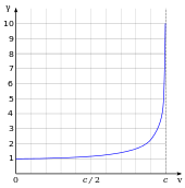
γ starts at 1 when v equals zero and stays nearly constant for small v's, then it sharply curves upwards and has a vertical asymptote, diverging to positive infinity as v approaches c.
The Lorentz factor γ as a function of velocity. It starts at 1 and approaches infinity as v approaches c.

Special relativity has many counter-intuitive implications, which have been verified in many experiments.[17] These include the equivalence of mass and energy (E = mc2), length contraction (moving objects shorten),[Note 4] and time dilation (moving clocks run slower). The factor γ by which lengths contract and times dilate, known as the Lorentz factor, is given by γ = (1 − v2/c2)−1/2, where v is the speed of the object; its difference from 1 is negligible for speeds much slower than c, such as most everyday speeds—in which case special relativity is closely approximated by Galilean relativity—but it increases at relativistic speeds and diverges to infinity as v approaches c.

Three pairs of coordinate axes are depicted with the same origin A; in the green frame, the x axis is horizontal and the ct axis is vertical; in the red frame, the x′ axis is slightly skewed upwards, and the ct′ axis slightly skewed rightwards, relative to the green axes; in the blue frame, the x′′ axis is somewhat skewed downwards, and the ct′′ axis somewhat skewed leftwards, relative to the green axes. A point B on the green x axis, to the left of A, has zero ct, positive ct′, and negative ct′′.
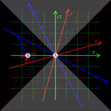
Event A precedes B in the red frame, is simultaneous with B in the green frame, and follows B in the blue frame.

Another counter-intuitive consequence of special relativity is the relativity of simultaneity: if the spatial distance between two events A and B is greater than the time interval between them multiplied by c, then there are frames of reference in which A precedes B, others in which B precedes A, and others in which they are simultaneous; neither event can be the cause of the other.

The results of special relativity can be summarized by treating space and time as a unified structure known as spacetime (with c relating the units of space and time), and requiring that physical theories satisfy a special symmetry called Lorentz invariance, whose mathematical formulation contains the parameter c.[20] Lorentz invariance has become an almost universal assumption for modern physical theories, such as quantum electrodynamics, quantum chromodynamics, the Standard Model of particle physics, and general relativity. As such, the parameter c is ubiquitous in modern physics, appearing in many contexts that may seem to be unrelated to light. For example, general relativity predicts that c is also the speed of gravity and of gravitational waves.[21]

In non-inertial frames of reference (gravitationally curved space or accelerated reference frames), the local speed of light is constant and equal to c, but the speed of light along a trajectory of finite length can differ from c, depending on how distances and times are defined.[22]

It is generally assumed in physics that fundamental constants such as c have the same value throughout spacetime, meaning that they do not depend on location and do not vary with time. However, various theories have suggested that the speed of light has changed over time.[23][24] Although no conclusive evidence for such theories has been found, they remain the subject of ongoing research.[25][26][27]

Upper limit on speeds

According to special relativity, the energy of an object with rest mass m and speed v is given by γmc2, where γ is the Lorentz factor defined above. When v is zero, γ is equal to one, giving rise to the famous E = mc2 formula for mass-energy equivalence. Since the γ factor approaches infinity as v approaches c, it would take an infinite amount of energy to accelerate an object with mass to the speed of light. The speed of light is the upper limit for the speeds of objects with positive rest mass.[28]

More generally, it is normally impossible for any information or energy to travel faster than c. One reason is that according to the theory of special relativity, if something were travelling faster than c relative to an inertial frame of reference, it would be travelling backwards in time relative to another frame,[Note 5] and causality would be violated.[Note 6][30] In such a frame of reference, an "effect" could be observed before its "cause". Such a violation of causality has never been recorded,[14] and would lead to paradoxes.[Note 7][31] Faster-than-light observations and experiments

There are situations in which it may seem that matter, energy, or information travels at speeds greater than c, but they do not. For example, if a laser beam is swept quickly across a distant object, the spot of light can move faster than c, but the only physical entities that are moving are the laser and its emitted light, which travels at the speed c from the laser to the various positions of the spot. The movement of the spot will be delayed after the laser is moved because of the time it takes light to get to the distant object from the laser. Similarly, a shadow projected onto a distant object can be made to move faster than c.[32] In neither case does any matter or information travel faster than light.[33]

In some interpretations of quantum mechanics, certain quantum effects may seem to be transmitted faster than c—and thus instantaneously in some frame—as in the EPR paradox. An example involves the quantum states of two particles that can be entangled. Until either of the particles is observed, they exist in a superposition of two quantum states. If the particles are separated and one particle's quantum state is observed, the other particle's quantum state is determined instantaneously (i.e., faster than light could travel from one particle to the other). However, it is impossible to control which quantum state the first particle will take on when it is observed, so information cannot be transmitted in this manner.[33][34]

Another quantum effect that predicts the occurrence of faster-than-light speeds is called the Hartman effect; under certain conditions the time needed for a particle to tunnel through a barrier is constant.[35][36] This could result in a particle crossing a large gap faster-than-light. However, no information can be sent using this effect.[37]

As is discussed in the propagation of light in a medium section below, many wave velocities can exceed c. For example, the phase velocity of X-rays through most glasses can routinely exceed c,[38] but such waves cannot convey any information.[39]

The rate of change in the distance between two objects in a frame of reference with respect to which both are moving (their closing speed) may have a value in excess of c. However, this does not represent the speed of any single object as measured in a single inertial frame.[citation needed]

So-called superluminal motion is seen in certain astronomical objects,[40] such as the relativistic jets of radio galaxies and quasars. However, these jets are not moving at speeds in excess of the speed of light: the apparent superluminal motion is a projection effect caused by objects moving near the speed of light and approaching Earth at a small angle to the line of sight: since the light which was emitted when the jet was farther away took longer to reach the Earth, the time between two successive observations corresponds to a longer time between the instants at which the light rays were emitted.[41]

In models of the expanding universe, the farther galaxies are from each other, the faster they drift apart. This receding is not due to motion through space, but rather to the expansion of space itself.[33] For example, galaxies far away from Earth appear to be moving away from the Earth with a speed proportional to their distances. Beyond a boundary called the Hubble sphere, this apparent recessional velocity becomes greater than the speed of light.[42]

Propagation of light

In classical physics, light is described as a type of electromagnetic wave. The classical behaviour of the electromagnetic field is described by Maxwell's equations, which predict that the speed c with which electromagnetic waves (such as light) propagate through the vacuum is related to the electric constant ε0 and the magnetic constant μ0 by the equation c = 1/ε0μ0.[43]

In modern quantum physics, the electromagnetic field is described by the theory of quantum electrodynamics (QED). In this theory, light is described by the fundamental excitations (or quanta) of the electromagnetic field, called photons. In QED, photons are massless particles and thus, according to special relativity, they must travel at the speed of light.

Extensions of QED in which the photon has a mass have been considered. In such a theory, its speed would depend on its frequency, and the invariant speed c of special relativity would then be the upper limit of the speed of light in vacuum.[22] To date no such effects have been observed,[44][45][46] putting stringent limits on the mass of the photon. The limit obtained depends on the used model: if the massive photon is described by Proca theory,[47] the experimental upper bound for its mass is about 10−57 grams;[48] if photon mass is generated by a Higgs mechanism, the experimental upper limit is less sharp, m ≤ 10−14 eV/c2 [47] (roughly 2 × 10−47 g).

Another reason for the speed of light to vary with its frequency would be the failure of special relativity to apply to arbitrarily small scales, as predicted by some proposed theories of quantum gravity. In 2009, the observation of the spectrum of gamma-ray burst GRB 090510 did not find any difference in the speeds of photons of different energies, confirming that Lorentz invariance is verified at least down to the scale of the Planck length (lP = ħG/c31.6163×10−35 m) divided by 1.2.[49]

In a medium

When light enters materials, its energy is absorbed. In the case of transparent materials, this energy is quickly re-radiated. However, this absorption and re-radiation introduces a delay. As light propagates through dielectric material it undergoes continuous absorption and re-radiation. Therefore the speed of light in a medium is said to be less than c, which should be read as the speed of energy propagation at the macroscopic level. At an atomic level, electromagnetic waves always travel at c in the empty space between atoms. Two factors influence this slowing: stronger absorption leading to shorter path length between each re-radiation cycle, and longer delays. The slowing is therefore the result of these two factors.[50] The refractive index of a transparent material is defined as the ratio of c to the speed of light v in the material. Larger indices of refraction indicate smaller speeds. The refractive index of a material may depend on the light's frequency, intensity, polarization, or direction of propagation. In many cases, though, it can be treated as a material-dependent constant. The refractive index of air is approximately 1.0003.[51] Denser media, such as water and glass, have refractive indexes of around 1.3 and 1.5 respectively for visible light.[52]Diamond has a refractive index of about 2.4.[53]

A white beam of light enters a prism and a spectrum comes out of it.
The light passing through a dispersive prism demonstrates refraction and, by the splitting of white light into a spectrum of colors, dispersion.

If the refractive index of a material depends on the frequency of the light passing through the medium, there exist two notions of the speed of light in the medium. One is the speed of a wave of a single frequency f. This is called the phase velocity vp(f), and is related to the frequency-dependent refractive index n(f) by vp(f) = c/n(f). The other is the average velocity of a pulse of light consisting of different frequencies of light. This is called the group velocity and not only depends on the properties of the medium but also the distribution of frequencies in the pulse. A pulse with different group and phase velocities is said to undergo dispersion.

Certain materials have an exceptionally low group velocity for light waves, a phenomenon called slow light. In 1999, a team of scientists led by Lene Hau were able to slow the speed of a light pulse to about 17 metres per second (61 km/h; 38 mph);[54] in 2001, they were able to momentarily stop a beam.[55] In 2003, scientists at Harvard University and the Lebedev Physical Institute in Moscow, succeeded in completely halting light by directing it into a Bose–Einstein condensate of the element rubidium, the atoms of which, in Lukin's words, behaved "like tiny mirrors" due to an interference pattern in two "control" beams.[56][57]

It is also possible for the group velocity of light pulses to exceed c.[58] In an experiment in 2000, laser beams travelled for extremely short distances through caesium atoms with a group velocity of 300 times c.[59] It is not possible to transmit information faster than c by this means because the speed of information transfer cannot exceed the front velocity of the wave pulse, which is always less than c.[60] The requirement that causality is not violated implies that the real and imaginary parts of the dielectric constant of any material, corresponding respectively to the index of refraction and to the attenuation coefficient, are linked by the Kramers–Kronig relations.[61]

Practical effects of finiteness

The finiteness of the speed of light has implications for various sciences and technologies. For some it creates challenges or limits: for example, c, being the upper limit of the speed with which signals can be sent, provides a theoretical upper limit for the operating speed of microprocessors. For others it creates opportunities, for example to measure distances.

The speed of light is of relevance to communications. For example, given the equatorial circumference of the Earth is about 40,075 km and c about 300,000 km/s, the theoretical shortest time for a piece of information to travel half the globe along the surface is about 67 milliseconds. When light is traveling around the globe in an optical fiber, the actual transit time is longer, in part because the speed of light is slower by about 35% in an optical fiber, depending on its refractive index n.[62] Furthermore, straight lines rarely occur in global communications situations, and delays are created when the signal passes through an electronic switch or signal regenerator.[63]

The diameter of the moon is about one quarter of that of Earth, and their distance is about thirty times the diameter of Earth. A beam of light starts from the Earth and reaches the Moon in about a second and a quarter.
A beam of light is depicted travelling between the Earth and the Moon in the same time it takes light to scale the distance between them: 1.255 seconds at its mean orbital (surface to surface) distance. The relative sizes and separation of the Earth–Moon system are shown to scale.

Another consequence of the finite speed of light is that communications between the Earth and spacecraft are not instantaneous. There is a brief delay from the source to the receiver, which becomes more noticeable as distances increase. This delay was significant for communications between ground control and Apollo 8 when it became the first manned spacecraft to orbit the Moon: for every question, the ground control station had to wait at least three seconds for the answer to arrive.[64] The communications delay between Earth and Mars is almost ten minutes. As a consequence of this, if a robot on the surface of Mars were to encounter a problem, its human controllers would not be aware of it until ten minutes later; it would then take at least a further ten minutes for instructions to travel from Earth to Mars.

The speed of light can also be of concern over very short distances. In supercomputers, the speed of light imposes a limit on how quickly data can be sent between processors. If a processor operates at 1 gigahertz, a signal can only travel a maximum of about 30 centimetres (1 ft) in a single cycle. Processors must therefore be placed close to each other to minimize communication latencies, which can cause difficulty with cooling. If clock frequencies continue to increase, the speed of light will eventually become a limiting factor for the internal design of single chips.[65]

Distance measurement

Radar systems measure the distance to a target by the time it takes a radio-wave pulse to return to the radar antenna after being reflected by the target: the distance to the target is half the round-trip transit time multiplied by the speed of light. A Global Positioning System (GPS) receiver measures its distance to GPS satellites based on how long it takes for a radio signal to arrive from each satellite, and from these distances calculates the receiver's position. Because light travels about 300,000 kilometres (186,000 miles) in one second, these measurements of small fractions of a second must be very precise. The Lunar Laser Ranging Experiment, radar astronomy and the Deep Space Network determine distances to the Moon, planets and spacecraft, respectively, by measuring round-trip transit times.

Astronomy

The finite speed of light is important in astronomy. Due to the vast distances involved, it can take a very long time for light to travel from its source to Earth. For example, it has taken 13 billion (13 × 109) years for light to travel to Earth from the faraway galaxies viewed in the Hubble Ultra Deep Field images.[66][67] Those photographs, taken today, capture images of the galaxies as they appeared 13 billion years ago, when the universe was less than a billion years old.[66] The fact that farther-away objects appear younger (due to the finite speed of light) allows astronomers to infer the evolution of stars, of galaxies, and of the universe itself.

Astronomical distances are sometimes expressed in light-years, especially in popular science publications.[68] A light‑year is the distance light travels in one year, around 9461 billion kilometres, 5879 billion miles, or 0.3066 parsecs. Proxima Centauri, the closest star to Earth after the Sun, is around 4.2 light‑years away.[69]

Measurement

To measure the speed of light, various methods can be used which involve observation of astronomical phenomena or experimental setups on Earth. The setups could use mechanical devices (e.g. toothed wheels), optics (e.g. beam splitters, lenses and mirrors), electro-optics (e.g. lasers), or electronics in conjunction with a cavity resonator.

Astronomical measurements

Due to the large scale and the vacuum of space observations in the solar system and in astronomy in general provide a natural setting for measuring the speed of light. The result of such a measurement usually appears as the time needed for light to transverse some reference distance in the solar system such as the radius of the Earth's orbit. Historically such measurements could be made fairly accurately, compared to how accurate the length of the reference distance is known in Earth-based units. As such, it is customary to express the results in astronomical units per day. An astronomical unit is approximately equal to the average distance between the Earth and the Sun.[Note 8] Since the most used reference length scale in modern experiments (the SI metre) is determined by the speed of light, the value of c is fixed when measured in metres per second. Measurements of c in astronomical units provides an independent alternative to measure c.

One such method was used by Ole Christensen Rømer to provide the first quantitative estimate of the speed of light.[71][72] When observing the periods of moons orbiting a distant planet these periods appear to be shorter when the Earth is approaching that planet than when the Earth is receding from it. This effect occurs because the Earth's movement causes the path travelled by light from the planet to Earth to shorten (or lengthen respectively). The observed change in period is the time needed by light to cover the difference in path length. Rømer observed this effect for Jupiter's innermost moon Io and deduced from it that light takes 22 minutes to cross the diameter of the Earth's orbit.

A star emits a light ray which hits the objective of a telescope. While the light travels down the telescope to its eyepiece, the telescope moves to the right. For the light to stay inside the telescope, the telescope must be tilted to the right, causing the distant source to appear at a different location to the right.
Aberration of light: light from a distant source will appear to a different location for a moving telescope due to the finite speed of light.

Another method is to use the aberration of light, discovered and explained by James Bradley in the 18th century.[73] This effect results from the vector addition of the velocity of light arriving from a distant source (such as a star) and the velocity of its observer (see diagram on the left). A moving observer thus sees the light coming from a slightly different direction and consequently sees the source at a position shifted from its original position. Since the direction of the Earth's velocity changes continuously as the Earth orbits the Sun, this effect causes the apparent position of stars to move around. From the angular difference in the position of stars (maximally 20.5 arcseconds)[74] it is possible to express the speed of light in terms of the Earth's velocity around the Sun, which with the known length of a year can be easily converted in the time needed to travel from the Sun to Earth. In 1729, Bradley used this method to derive that light travelled 10,210 times faster than the Earth in its orbit (the modern figure is 10,066 times faster) or, equivalently, that it would take light 8 minutes 12 seconds to travel from the Sun to the Earth.[73]

Nowadays, the "light time for unit distance"—the inverse of c, expressed in seconds per astronomical unit—is measured by comparing the time for radio signals to reach different spacecraft in the Solar System, with their position calculated from the gravitational effects of the Sun and various planets. By combining many such measurements, a best fit value for the light time per unit distance is obtained. As of 2009, the best estimate, as approved by the International Astronomical Union (IAU), is:[75][76][77]

light time for unit distance: 499.004783836(10) s
c = 0.00200398880410(4) AU/s = 173.144632674(3) AU/day

The relative uncertainty in these measurements is 0.02 parts per billion (2 × 10⁻¹¹), equivalent to the uncertainty in Earth-based measurements of length by interferometry.[78][79] Since the meter is defined to be the length travelled by light in a certain time interval, the measurement of the light time for unit distance can also be interpreted as measuring the length of an AU in meters.

Time of flight techniques

A method of measuring the speed of light is to measure the time needed for light to travel to a mirror at a known distance and back. This is the working principle behind the Fizeau–Foucault apparatus developed by Hippolyte Fizeau and Léon Foucault.

A light ray passes horizontally through a half-mirror and a rotating cog wheel, is reflected back by a mirror, passes through the cog wheel, and is reflected by the half-mirror into a monocular.
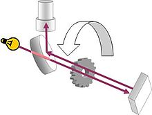
Diagram of the Fizeau apparatus

The setup as used by Fizeau consists of a beam of light directed at a mirror 8 kilometres (5 mi) away. On the way from the source to the mirror, the beam passes through a rotating cogwheel. At a certain rate of rotation, the beam passes through one gap on the way out and another on the way back, but at slightly higher or lower rates, the beam strikes a tooth and does not pass through the wheel. Knowing the distance between the wheel and the mirror, the number of teeth on the wheel, and the rate of rotation, the speed of light can be calculated.[80]

The method of Foucault replaces the cogwheel by a rotating mirror. Because the mirror keeps rotating while the light travels to the distant mirror and back, the light is reflected from the rotating mirror at a different angle on its way out than it is on its way back. From this difference in angle, the known speed of rotation and the distance to the distant mirror the speed of light may be calculated.[81]

Nowadays, using oscilloscopes with time resolutions of less than one nanosecond, the speed of light can be directly measured by timing the delay of a light pulse from a laser or an LED reflected from a mirror. This method is less precise (with errors of the order of 1%) than other modern techniques, but it is sometimes used as a laboratory experiment in college physics classes.[82][83][84]

Electromagnetic constants

An option for measuring c that does not directly depend on the propagation of electromagnetic waves is to use relation between c and the vacuum permittivity ε0 vacuum permeability μ0 established by Maxwell theory: c2 = 1/ε0μ0. The vacuum permittivity may be determined by measuring the capacitance and dimensions of a capacitor, whereas the value of the vacuum permeability is fixed at exactly ×10−7 H·m−1 through the definition of the ampere. Rosa and Dorsey used this method in 1907 to find a value of 299,710±22 km/s.[85][86]

Cavity resonance

A box with three waves in it; there are one and a half wavelength of the top wave, one of the middle one, and a half of the bottom one.
Electromagnetic standing waves in a cavity.

Another way to measure the speed of light is to independently measure the frequency f and wavelength λ of an electromagnetic wave in vacuum. The value of c can then be found by using the relation c = . One option is to measure the resonance frequency of a cavity resonator. If the dimensions of the resonance cavity are also known, these can be used determine the wavelength of the wave. In 1946, Louis Essen and A.C. Gordon-Smith establish the frequency for a variety of normal modes of microwaves of a microwave cavity of precisely known dimensions. As the wavelength of the modes was known from the geometry of the cavity and from electromagnetic theory, knowledge of the associated frequencies enabled a calculation of the speed of light.[85][87]

The Essen–Gordon-Smith result, 299,792±9 km/s, was substantially more precise than those found by optical techniques.[85] By 1950, repeated measurements by Essen established a result of 299,792.5±3.0 km/s.[88]

A household demonstration of this technique is possible, using a microwave oven and food such as marshmallows or margarine: if the turntable is removed so that the food does not move, it will cook the fastest at the antinodes (the points at which the wave amplitude is the greatest), where it will begin to melt. The distance between two such spots is half the wavelength of the microwaves; by measuring this distance and multiplying the wavelength by the microwave frequency (usually displayed on the back of the oven, typically 2450 MHz), the value of c can be calculated, "often with less than 5% error".[89][90]

Laser interferometry

An alternative to the cavity resonator method to find the wavelength for determining the speed of light is to use a form of interferometer.[91] A coherent light beam with a known frequency (f), as from a laser, is split to follow two paths and then recombined. By carefully changing the path length and observing the interference pattern, the wavelength of the light (λ) can be determined, which is related to the speed of light by the equation c = λf.

The main difficulty in measuring c through interferometry is to measure the frequency of light in or near the optical region; such frequencies are too high to be measured with conventional methods. This was first overcome by a group at the US National Institute of Standards and Technology (NIST) laboratories in Boulder, Colorado, in 1972.[92] By a series of photodiodes and specially constructed metal–insulator–metal diodes, they succeeded in linking the frequency of a methane-stabilized infrared laser to the frequency of the caesium transition used in atomic clocks (nearly 10,000 times lower, in the microwave region).[93] Their results for the frequency and wavelength of the infrared laser, and the resulting value for c, were:

f = 88.376181627±0.000000050 THz;
λ = 3.392231376±0.000000012 µm;
c = 299,792,456.2±1.1 m/s;

nearly a hundred times more precise than previous measurements of the speed of light.[92][93]

History

Until the early modern period, it was not known whether light travelled instantaneously or at a finite speed. The first extant recorded examination of this subject was in ancient Greece. Empedocles was the first to claim that the light has a finite speed.[94] He maintained that light was something in motion, and therefore must take some time to travel. Aristotle argued, to the contrary, that "light is due to the presence of something, but it is not a movement".[95] Euclid and Ptolemy advanced the emission theory of vision, where light is emitted from the eye, thus enabling sight. Based on that theory, Heron of Alexandria argued that the speed of light must be infinite because distant objects such as stars appear immediately upon opening the eyes.

Early Islamic philosophers initially agreed with the Aristotelian view that light had no speed of travel. In 1021, Islamic physicist Alhazen (Ibn al-Haytham) published the Book of Optics, in which he used experiments related to the camera obscura to support the now accepted intromission theory of vision, in which light moves from an object into the eye.[96] This led Alhazen to propose that light must therefore have a finite speed,[95][97][98] and that the speed of light is variable, decreasing in denser bodies.[98][99] He argued that light is a "substantial matter", the propagation of which requires time "even if this is hidden to our senses".[100]

Also in the 11th century, Abū Rayhān al-Bīrūnī agreed that light has a finite speed, and observed that the speed of light is much faster than the speed of sound.[101] Roger Bacon argued that the speed of light in air was not infinite, using philosophical arguments backed by the writing of Alhazen and Aristotle.[102][103] In the 1270s, Witelo considered the possibility of light travelling at infinite speed in a vacuum, but slowing down in denser bodies.[104]

In the early 17th century, Johannes Kepler believed that the speed of light was infinite, since empty space presents no obstacle to it. René Descartes argued that if the speed of light were finite, the Sun, Earth, and Moon would be noticeably out of alignment during a lunar eclipse. Since such misalignment had not been observed, Descartes concluded the speed of light was infinite. Descartes speculated that if the speed of light were found to be finite, his whole system of philosophy might be demolished.[95]

First measurement attempts

In 1629, Isaac Beeckman proposed an experiment in which a person would observe the flash of a cannon reflecting off a mirror about one mile (1.6 km) away. In 1638, Galileo Galilei proposed an experiment, with an apparent claim to having performed it some years earlier, to measure the speed of light by observing the delay between uncovering a lantern and its perception some distance away. He was unable to distinguish whether light travel was instantaneous or not, but concluded that if it weren't, it must nevertheless be extraordinarily rapid.[105][106] Galileo's experiment was carried out by the Accademia del Cimento of Florence, Italy, in 1667, with the lanterns separated by about one mile, but no delay was observed. Based on the modern value of the speed of light, the actual delay in this experiment would be about 11 microseconds. Robert Hooke explained the negative results as Galileo had by pointing out that such observations did not establish the infinite speed of light, but only that the speed must be very great.

A diagram of a planet's orbit around the Sun and of a moon's orbit around another planet. The shadow of the latter planet is shaded.
Rømer's observations of the occultations of Io from Earth

The first quantitative estimate of the speed of light was made in 1676 by Ole Christensen Rømer (see Rømer's determination of the speed of light).[71][72] From the observation that the periods of Jupiter's innermost moon Io appeared to be shorter when the earth was approaching Jupiter than when receding from it, he concluded that light travels at a finite speed, and was able to estimate that would take light 22 minutes to cross the diameter of Earth's orbit. Christiaan Huygens combined this estimate with an estimate for the diameter of the Earth's orbit to obtain an estimate of speed of light of 220,000 km/s, 26% lower than the actual value.[107]

In his 1704 book Opticks, Isaac Newton reported Rømer's calculations of the finite speed of light and gave a value of "seven or eight minutes" for the time taken for light to travel from the Sun to the Earth (the modern value is 8 minutes 19 seconds).[108] Newton queried whether Rømer's eclipse shadows were coloured; hearing that they weren't, he concluded the different colours travelled at the same speed. In 1729, James Bradley discovered the aberration of light.[73] From this effect he determined that light must travel 10,210 times faster than the Earth in its orbit (the modern figure is 10,066 times faster) or, equivalently, that it would take light 8 minutes 12 seconds to travel from the Sun to the Earth.[73]

19th and early 20th century

In the 19th century Hippolyte Fizeau developed a method to determine the speed of light based on time-of-flight measurements on Earth and reported a value of 315,000 km/s. His method was improved upon by Léon Foucault who obtained a value of 298,000 km/s in 1862.[80] James Clerk Maxwell observed that this value was very close to the parameter c appearing in his theory of electromagnetism as the propagation speed of the electromagnetic field, and suggested that light was an electromagnetic wave.[109]

It was thought at the time that electromagnetic field existed in some background medium called the luminiferous aether. This aether acted as an absolute reference frame for all physics and should be possible to measure the motion of the Earth with respect to this medium. In the second half of the 19th century and the beginning of the 20th century several experiments were performed to try to detect this motion, the most famous of which is the experiment performed by Albert Michelson and Edward Morley in 1887.[110] None of the experiments found any hint of the motion, finding that the speed of light was the same in every direction.[111]

In 1905 Albert Einstein proposed that the speed of light was independent of the motion of the source or observer. Using this and the principle of relativity as a basis he derived his special theory of relativity, in which the speed of light c featured as a fundamental parameter, also appearing in contexts unrelated to light.[112]

Increased accuracy and redefinition of the metre

History of measurements of c
Year Author and method Value (km/s)
1675 Rømer and Huygens, moons of Jupiter 220,000[72][107]
1729 James Bradley, aberration of light 301,000
1849 Hippolyte Fizeau, toothed wheel 315,000
1862 Léon Foucault, rotating mirror 298,000±500
1907 Rosa and Dorsay, EM constants 299,788±30
1926 Albert Michelson, rotating mirror 299,796±4
1947 Essen and Gordon-Smith, cavity resonator 299,792±3
1958 K.D. Froome, radio interferometry 299,792.5±0.1
1973 Evanson et al., laser interferometry 299,792.4574±0.001
1983 17th CGPM, definition of the metre 299,792.458 (exact)

In the second half of the 20th century much progress was made in increasing the accuracy of measurements of the speed of light, first by cavity resonance techniques and later by laser interferometer techniques. In 1972, using the latter method, a team at the US National Institute of Standards and Technology (NIST) laboratories in Boulder, Colorado determined the speed of light to be c = 299,792,456.2±1.1 m/s.[92][93] Almost all the uncertainty in this measurement of the speed of light was due to uncertainty in the length of the metre.[93][92][113] Since 1960, the metre had been defined as a given number of wavelengths of the light of one of the spectral lines of krypton,[Note 9] but it turned out that the chosen spectral line was not perfectly symmetrical.[93] This made its wavelength, and hence the length of the metre, uncertain, because the definition did not specify what point on the line profile (e.g., its maximum-intensity point or its centre of gravity) it referred to.[Note 10]

To get around this problem, in 1975, the 15th Conférence Générale des Poids et Mesures (CGPM) recommended using 299,792,458 metres per second for "the speed of propagation of electromagnetic waves in vacuum".[113] Based on this recommendation, the 17th CGPM in 1983 redefined the metre as "the length of the path travelled by light in vacuum during a time interval of 1299,792,458 of a second".[115]

The effect of this definition gives the speed of light the exact value 299,792,458 m/s, which is nearly the same as the value 299,792,456.2±1.1 m/s obtained in the 1972 experiment. The CGPM chose this value to minimise any change in the length of the metre.[116][117] As a result, in the SI system of units the speed of light is now a defined constant.[7] Improved experimental techniques do not affect the value of the speed of light in SI units, but do result in a more precise realisation of the SI metre.[118][119]
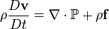